Improving Performance¶

Overview¶

This section covers the main strategies for making spinterp faster:

Vectorising the objective function
Reusing previously computed results
Purging redundant interpolant data
Vectorised interpolant evaluation

Vectorising the objective function¶

Vectorisation is most beneficial when function evaluations are cheap (\(\lesssim 10^{-2}\) s each). Consider the function

\[ f(x_1, x_2) = (x_1\, x_2)^2. \]

A non-vectorised implementation evaluates one point at a time:

def f(x1, x2):
    return (x1 * x2) ** 2

A vectorised implementation processes a whole array in one call:

import numpy as np
def f_vec(x1, x2):
    return (x1 * x2) ** 2      # NumPy broadcasts automatically

When passing a vectorised function, the grid points are delivered as full arrays, avoiding per-point Python call overhead. For cheap functions, this can give a 2× or better speed-up when computing surpluses.

Reusing previous results¶

The hierarchical surplus structure means that a higher-level interpolant is a strict extension of a lower-level one. You never need to recompute previously computed levels.

The recommended pattern is to build the interpolant in a loop, checking the estimated error after each level:

import numpy as np
import spinterp

def f_vec(x1, x2):
    return (x1 * x2) ** 2

d, n_max = 2, 8
all_seq, all_surp = [], []
est_err = np.inf

for k in range(n_max + 1):
    nl  = spinterp.spnlevels(k, d)
    seq = spinterp.spgetseq(k, d, nl)
    tp  = spinterp.spdim_cc(seq)
    x_k = spinterp.spgrid_cc(seq, tp)
    fvals = np.array([f_vec(*x_k[i]) for i in range(tp)])

    if k == 0:
        surp = fvals.copy()
    else:
        z_prev   = np.concatenate(all_surp)
        seq_prev = np.vstack(all_seq)
        surp = fvals - spinterp.spcmpvals_cc(z_prev, x_k, seq, seq_prev)

    all_seq.append(seq)
    all_surp.append(surp)

    # Estimated error = max |surplus| / (max |f| + eps)
    est_err = np.max(np.abs(surp)) / (np.max(np.abs(fvals)) + 1e-14)
    print(f"level {k}: {tp} new pts, est. rel. error = {est_err:.3e}")

    if est_err < 1e-4:
        break

Example output for a smooth function:

level 0:    1 new pts, est. rel. error = 1.000e+00
level 1:    4 new pts, est. rel. error = 3.750e-01
level 2:    8 new pts, est. rel. error = 4.688e-02
level 3:   16 new pts, est. rel. error = 2.930e-03
level 4:   28 new pts, est. rel. error = 8.545e-05

Purging interpolant data¶

After the interpolant is built, subgrids whose hierarchical surpluses are all below a drop tolerance can be excluded from evaluation without significantly affecting accuracy. This is the sppurge concept from the original MATLAB toolbox.

A simple Python equivalent: keep only subgrids where \(|\alpha_{\mathbf{l}}|_\infty\) exceeds a threshold:

import numpy as np
import spinterp

d         = 2
max_level = 6

def f(x, y):
    return np.sin(x) + np.cos(y)

# Build hierarchical surpluses (Clenshaw-Curtis grid)
all_seq, all_surp = [], []
for k in range(max_level + 1):
    nl  = spinterp.spnlevels(k, d)
    seq = spinterp.spgetseq(k, d, nl)
    tp  = spinterp.spdim_cc(seq)
    x_k = spinterp.spgrid_cc(seq, tp)
    fvals = np.array([f(*x_k[i]) for i in range(tp)])
    if k == 0:
        surp_k = fvals.copy()
    else:
        z_prev   = np.concatenate(all_surp)
        seq_prev = np.vstack(all_seq)
        surp_k   = fvals - spinterp.spcmpvals_cc(z_prev, x_k, seq, seq_prev)
    all_seq.append(seq)
    all_surp.append(surp_k)

# Purge subgrids whose surpluses are all below the drop tolerance
drop_tol = 1e-5
keep = [
    (s, surp)
    for s, surp in zip(all_seq, all_surp)
    if np.max(np.abs(surp)) > drop_tol
]
seq_pruned = np.vstack([s    for s, _    in keep])
z_pruned   = np.concatenate([surp for _, surp in keep])

print(f"Original subgrids: {len(all_seq)},  after purge: {len(keep)}")
print(f"Original surpluses: {sum(len(s) for s in all_surp)},  after purge: {len(z_pruned)}")

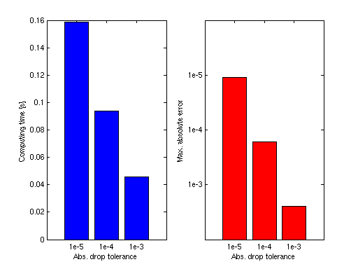
The trade-off: smaller drop_tol → higher accuracy, slower evaluation. Typical savings are 2–5× speedup at the cost of \(\sim 10^{-4}\) relative accuracy degradation when drop_tol = 1e-5.

Purging trade-off: computation time vs maximum error

Vectorised interpolant evaluation¶

The spinterp_cc (and related) functions are designed for batch evaluation: passing all query points as a single 2-D array is far more efficient than one-point-at-a-time calls.

import numpy as np
import spinterp

d         = 2
max_level = 4

def f(x, y):
    return np.sin(x) + np.cos(y)

# Build hierarchical surpluses (Clenshaw-Curtis grid)
all_seq, all_surp = [], []
for k in range(max_level + 1):
    nl  = spinterp.spnlevels(k, d)
    seq = spinterp.spgetseq(k, d, nl)
    tp  = spinterp.spdim_cc(seq)
    x_k = spinterp.spgrid_cc(seq, tp)
    fvals = np.array([f(*x_k[i]) for i in range(tp)])
    if k == 0:
        surp_k = fvals.copy()
    else:
        z_prev   = np.concatenate(all_surp)
        seq_prev = np.vstack(all_seq)
        surp_k   = fvals - spinterp.spcmpvals_cc(z_prev, x_k, seq, seq_prev)
    all_seq.append(seq)
    all_surp.append(surp_k)

z   = np.concatenate(all_surp)
seq = np.vstack(all_seq)

rng = np.random.default_rng(0)
pts = rng.random((1000, d))

# Slow — Python loop over 1000 points
results_slow = [spinterp.spinterp_cc(z, pts[i:i+1], seq)[0] for i in range(1000)]

# Fast — single batched call
results_fast = spinterp.spinterp_cc(z, pts, seq)   # pts.shape = (1000, d)

print(f"Max diff slow vs fast: {np.max(np.abs(np.array(results_slow) - results_fast)):.2e}")

Typical speed-up: 50–100× for 1000 points, due to reduced Python overhead and better cache utilisation in the Fortran kernel.

Summary of tips¶

Tip	When to apply	Typical benefit
Vectorise the objective function	Cheap functions (\(< 10^{-2}\) s/eval)	2–10× faster `spcmpvals`
Build levels incrementally	Always	Avoids recomputing surpluses
Purge small-surplus subgrids	After convergence, if evaluation speed matters	2–5× faster `spinterp`
Batch query points	Always	50–100× faster `spinterp`
Use sparse index format	\(d > 10\)	Lower memory, faster iteration