Piecewise Linear Basis Functions
Piecewise linear basis functions provide a good compromise between accuracy and computational
cost due to their bounded support. spinterp includes three grid types that use
piecewise multilinear bases:
| Code name | Description |
|---|---|
clenshaw-curtis (CC) |
Nested boundary-point set; single node at level 0 |
maximum (M) |
Maximum-norm grid; \(3^d\) nodes at level 0 |
noboundary (NB) |
Interior-point grid; basis functions extrapolate towards boundary |
Hierarchical hat functions
In 1-D, the hat function centred at \(x_j\) with support width \(h\) is
For the Clenshaw-Curtis grid the 1-D nodes at level \(\ell\) are:
The NoBoundary grid uses only interior nodes \(x_j^{(\ell)} = (2j-1)/2^{\ell+1}\) for \(j = 1, \dots, 2^\ell\) at every level, with hat functions that extrapolate linearly past the boundary.
The hierarchical surplus \(\alpha_j\) at node \(x_j\) is the residual between the exact function value and the interpolant already built from coarser levels:
The full \(d\)-dimensional interpolant is then
where the outer sum runs over all active multi-indices \(\mathbf{l}\) in the Smolyak set.
Error estimate
For a function \(f\) that possesses bounded mixed partial derivatives of order 2 in each coordinate, i.e.
the interpolation error of the sparse grid \(A_{q,d}(f)\) in the maximum norm is
where \(N\) is the number of support nodes. The corresponding full-grid estimate with the same \(N^* \approx N\) nodes is only \(O(N^{*\,-2/d})\), which deteriorates rapidly with dimension. The sparse grid retains the \(N^{-2}\) rate, paying only a logarithmic price.
Grid point counts
The table below gives the number of grid points for the three piecewise-linear grid types.
| \(n\) | M (\(d=2\)) | NB (\(d=2\)) | CC (\(d=2\)) | M (\(d=4\)) | NB (\(d=4\)) | CC (\(d=4\)) | M (\(d=8\)) | NB (\(d=8\)) | CC (\(d=8\)) |
|---|---|---|---|---|---|---|---|---|---|
| 0 | 9 | 1 | 1 | 81 | 1 | 1 | 6561 | 1 | 1 |
| 1 | 21 | 5 | 5 | 297 | 9 | 9 | 41553 | 17 | 17 |
| 2 | 49 | 17 | 13 | 945 | 49 | 41 | 1.9e5 | 161 | 145 |
| 3 | 113 | 49 | 29 | 2769 | 209 | 137 | 7.7e5 | 1121 | 849 |
| 4 | 257 | 129 | 65 | 7681 | 769 | 401 | 2.8e6 | 6401 | 3937 |
| 5 | 577 | 321 | 145 | 20481 | 2561 | 1105 | 9.3e6 | 31745 | 15713 |
| 6 | 1281 | 769 | 321 | 52993 | 7937 | 2929 | 3.0e7 | 141569 | 56737 |
| 7 | 2817 | 1793 | 705 | 1.3e5 | 23297 | 7537 | 9.1e7 | 5.8e5 | 1.9e5 |
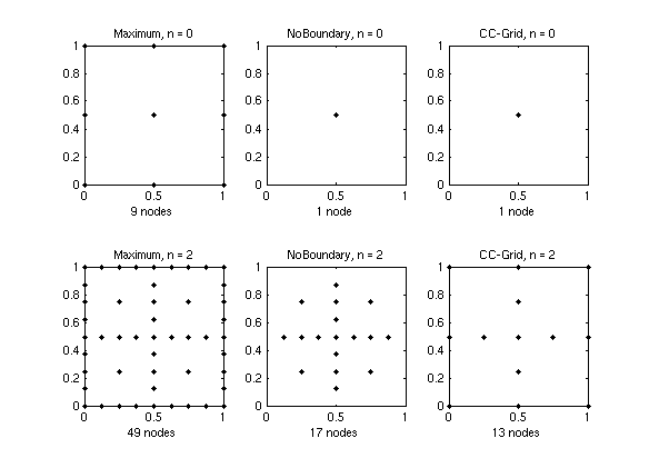
Visual comparison
The figure below shows the sparse grids of levels 0 and 2 for all three grid types in two dimensions.
Which grid type to choose?
-
Clenshaw-Curtis is the most versatile choice and the only grid type for which the dimension-adaptive algorithm is currently implemented. Recommended for most problems.
-
NoBoundary can outperform CC when the objective function is known to be non-zero at the domain boundary and the boundary nodes of CC do not contribute meaningful information.
-
Maximum has \(3^d\) nodes at level 0, making it impractical for \(d > 10\) (\(d = 10\) already requires 59049 nodes for the initial interpolant). Suitable only for low-dimensional problems.