Computing Derivatives¶

One primary purpose of sparse grid interpolation is constructing surrogate functions for local or global optimisation. spinterp computes exact derivatives of the interpolant — not finite-difference approximations — at almost no additional memory cost.

How to obtain derivatives¶

Call spderiv_cc (or spderiv_cb for the Chebyshev grid) instead of spinterp_cc. The function returns both the interpolated values and the full gradient vector:

import numpy as np
import spinterp

d = 2

def f(x, y):
    return np.sin(x) + np.cos(y)

# Build hierarchical surpluses (Clenshaw-Curtis grid)
all_seq, all_surp = [], []
for k in range(5):
    nl  = spinterp.spnlevels(k, d)
    seq = spinterp.spgetseq(k, d, nl)
    tp  = spinterp.spdim_cc(seq)
    x_k = spinterp.spgrid_cc(seq, tp)
    fvals = np.array([f(*x_k[i]) for i in range(tp)])
    if k == 0:
        surp_k = fvals.copy()
    else:
        z_prev   = np.concatenate(all_surp)
        seq_prev = np.vstack(all_seq)
        surp_k   = fvals - spinterp.spcmpvals_cc(z_prev, x_k, seq, seq_prev)
    all_seq.append(seq)
    all_surp.append(surp_k)

z   = np.concatenate(all_surp)
seq = np.vstack(all_seq)

pts_unit = np.array([[0.25, 0.4], [0.6, 0.75], [0.1, 0.9]])

# ip.shape  = (npoints,)
# grad.shape = (npoints, d)
ip, grad = spinterp.spderiv_cc(z, pts_unit, seq)
print("Values:  ", ip)
print("df/dx1:  ", grad[:, 0])
print("df/dx2:  ", grad[:, 1])

The procedure for building the surpluses z and level-index matrix seq is identical regardless of whether derivatives are needed.

Note

The computed derivatives are the exact derivatives of the interpolant (up to floating-point accuracy), not approximations of the derivatives of the original function \(f\). No additional memory is required.

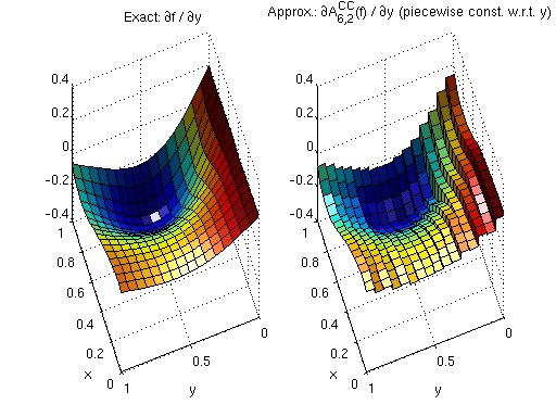
Derivatives of piecewise multilinear interpolants¶

Differentiating a piecewise linear function yields a piecewise constant function. The derivatives are exact everywhere except at the kinks (the grid nodes), where only a one-sided derivative exists.

Example — 2-D function¶

Consider the test function

\[ f(x, y) = \frac{1}{\cos^2(2x) + \sin^2(y) + 1} + 0.2\,y \]

with exact partial derivatives

\[ \frac{\partial f}{\partial x} = -\frac{4\cos(2x)\sin(2x)}{(\cos^2(2x) + \sin^2(y) + 1)^2}, \qquad \frac{\partial f}{\partial y} = \frac{-2\cos(y)\sin(y)}{(\cos^2(2x) + \sin^2(y) + 1)^2} + 0.2. \]

The figure below compares \(\partial f / \partial y\) (left, exact) with the sparse grid derivative \(\partial A^{\text{CC}}_{6,2}(f) / \partial y\) (right, piecewise constant with visible jumps at level-4 grid nodes):

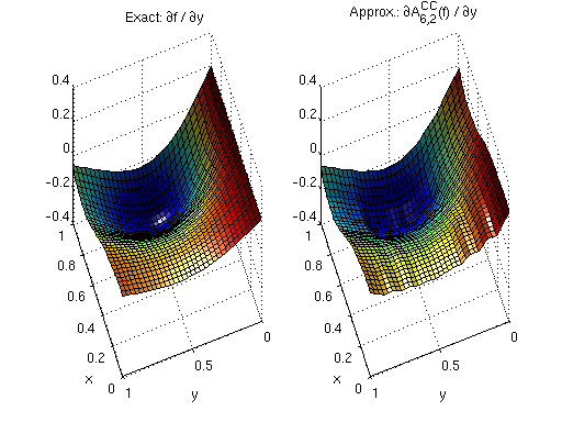
Exact vs piecewise-constant CC derivative

Augmented continuous derivatives¶

Discontinuous derivatives make first-order optimality conditions \(\nabla f = \mathbf{0}\) impossible to satisfy exactly, leading to slow convergence in gradient-based optimisation.

The continuous derivative option linearly interpolates the piecewise-constant derivative between two augmented evaluation points \(y_1\) and \(y_2\) on either side of each grid cell:

\[ \frac{\partial A}{\partial x_k}\bigg|_\text{cont}(y) = \frac{\partial A}{\partial x_k}(y_1) + \frac{\dfrac{\partial A}{\partial x_k}(y_2) - \dfrac{\partial A}{\partial x_k}(y_1)}{\Delta} (y - y_1) \]

where \(\Delta\) is the cell width \(1/2^{\ell_{\max}}\).

Use spcont_deriv_cc followed by pp_deriv to obtain continuous derivatives:

import numpy as np
import spinterp

d = 2

def f(x, y):
    return np.sin(x) + np.cos(y)

# Build hierarchical surpluses (Clenshaw-Curtis grid)
all_seq, all_surp = [], []
for k in range(5):
    nl  = spinterp.spnlevels(k, d)
    seq = spinterp.spgetseq(k, d, nl)
    tp  = spinterp.spdim_cc(seq)
    x_k = spinterp.spgrid_cc(seq, tp)
    fvals = np.array([f(*x_k[i]) for i in range(tp)])
    if k == 0:
        surp_k = fvals.copy()
    else:
        z_prev   = np.concatenate(all_surp)
        seq_prev = np.vstack(all_seq)
        surp_k   = fvals - spinterp.spcmpvals_cc(z_prev, x_k, seq, seq_prev)
    all_seq.append(seq)
    all_surp.append(surp_k)

z   = np.concatenate(all_surp)
seq = np.vstack(all_seq)

pts_unit  = np.array([[0.25, 0.4], [0.6, 0.75], [0.1, 0.9]])
maxlev    = int(seq.max())
maxlevvec = np.full(d, maxlev, dtype=np.int32)

ip, ipder, ipder2 = spinterp.spcont_deriv_cc(z, pts_unit, seq, maxlev)

# pp_deriv post-processes ipder in-place using ipder2
spinterp.pp_deriv(
    np.asfortranarray(ipder),
    np.asfortranarray(ipder2),
    maxlevvec,
    np.asfortranarray(pts_unit),
)
print("Values:   ", ip)
print("df/dx1:   ", ipder[:, 0])
print("df/dx2:   ", ipder[:, 1])

The figure below shows the same derivative after the continuity post-processing:

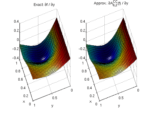
Continuous CC derivative after pp_deriv post-processing

Derivatives of polynomial interpolants¶

For the Chebyshev-Gauss-Lobatto grid, the basis functions are globally smooth polynomials. The derivatives are computed via the discrete cosine transform (DCT), using the spderiv_cb function:

import numpy as np
import spinterp

d = 2

def f(x, y):
    return np.sin(x) + np.cos(y)

# Build hierarchical surpluses (Chebyshev grid)
# CB uses the same point count as CC
all_seq, all_surp = [], []
for k in range(5):
    nl  = spinterp.spnlevels(k, d)
    seq = spinterp.spgetseq(k, d, nl)
    tp  = spinterp.spdim_cc(seq)
    x_k = spinterp.spgrid_cb(seq, tp)
    fvals = np.array([f(*x_k[i]) for i in range(tp)])
    if k == 0:
        surp_k = fvals.copy()
    else:
        z_prev   = np.concatenate(all_surp)
        seq_prev = np.vstack(all_seq)
        surp_k   = fvals - spinterp.spcmpvals_cb(z_prev, x_k, seq, seq_prev)
    all_seq.append(seq)
    all_surp.append(surp_k)

z_cb = np.concatenate(all_surp)
seq  = np.vstack(all_seq)

pts_unit = np.array([[0.25, 0.4], [0.6, 0.75], [0.1, 0.9]])

ip, grad = spinterp.spderiv_cb(z_cb, pts_unit, seq)
print("Values:  ", ip)
print("df/dx1:  ", grad[:, 0])
print("df/dx2:  ", grad[:, 1])

The resulting derivatives are infinitely smooth:

CGL polynomial derivative vs exact

Approximation quality¶

The figure below shows the maximum absolute error of the derivatives for six standard Genz test functions at 100 randomly sampled points for dimension \(d = 3\):

H\(^\text{CC}\) — piecewise constant, Clenshaw-Curtis grid
H\(^\text{CC}\) (cont.) — augmented continuous, Clenshaw-Curtis grid
H\(^\text{CGL}\) — smooth polynomial, Chebyshev grid

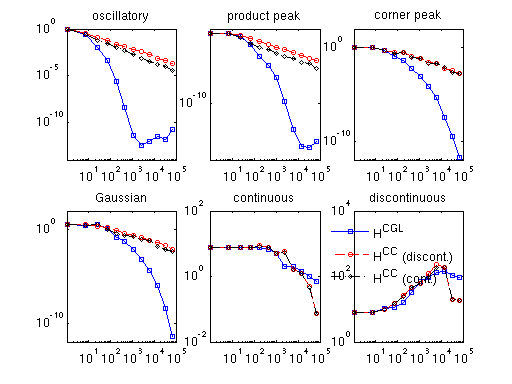
Derivative approximation quality comparison for d=3

Note

Functions with kinks (labelled continuous and discontinuous) cannot have their derivatives approximated in the maximum norm: convergence fails near the kinks. The error decreases in the plot only because the randomly sampled points are less likely to land near the (shrinking) non-convergent region.

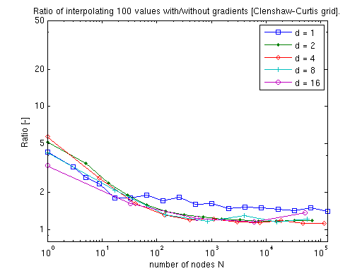
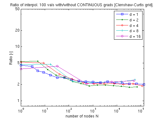
Computational cost¶

Clenshaw-Curtis¶

Computing the exact or augmented continuous gradient adds only a small, dimension-independent factor over plain interpolation:

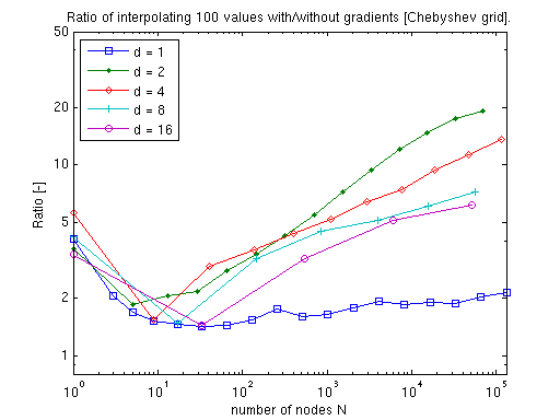
Timing: exact CC derivative Timing: continuous CC derivative

Chebyshev¶

The polynomial case requires more sophisticated algorithms. However, as the dimension increases, fewer subgrids need differentiation (lower-dimensional subgrids omit the dimensions they do not span), so the overhead decreases:

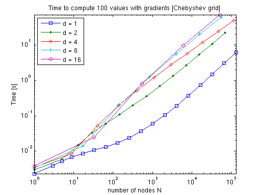
Timing: CGL derivative Timing: CGL derivative absolute

For comparison, numerical differentiation with a centred-difference formula would require \(2d + 1\) interpolant evaluations per gradient — the analytic approach is substantially cheaper for moderate to large \(d\).