Quick Start
A first example
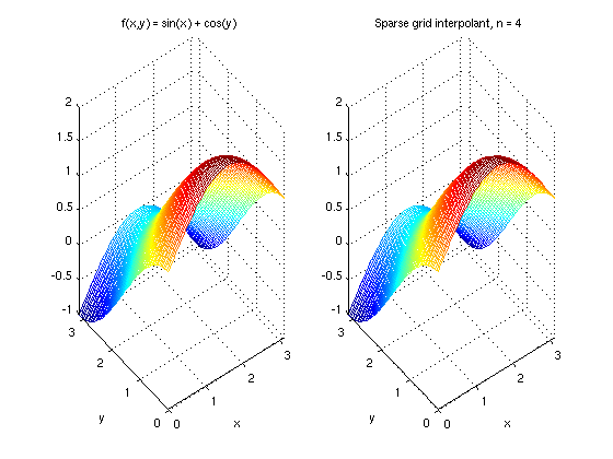
Consider interpolating the function
over the domain \([0, \pi] \times [0, \pi]\) using the default Clenshaw-Curtis sparse grid.
The complete script below builds the interpolant level by level, evaluates it at random points, computes gradient vectors, integrates over the domain, visualises the grid and the error surface, and demonstrates alternative grid types:
import numpy as np
import matplotlib.pyplot as plt
import spinterp

# ============================================================
# Problem setup
# ============================================================

d         = 2
max_level = 4
scale     = np.array([np.pi, np.pi])   # domain: [0, pi]^2

def f(x, y):
    return np.sin(x) + np.cos(y)

# ============================================================
# STEP 1 — Build hierarchical surpluses (Clenshaw-Curtis)
# ============================================================

all_seq  = []
all_surp = []

for k in range(max_level + 1):

    nl  = spinterp.spnlevels(k, d)
    seq = spinterp.spgetseq(k, d, nl)    # multi-index set, shape (nl, d)
    tp  = spinterp.spdim_cc(seq)          # total grid points at this level
    x_k = spinterp.spgrid_cc(seq, tp)    # sparse-grid points in [0,1]^d

    x_scaled = x_k * scale
    fvals    = np.array([
        f(x_scaled[i, 0], x_scaled[i, 1]) for i in range(tp)
    ])

    if k == 0:
        surp_k = fvals.copy()
    else:
        z_prev      = np.concatenate(all_surp)
        seq_prev    = np.vstack(all_seq)
        interp_prev = spinterp.spcmpvals_cc(z_prev, x_k, seq, seq_prev)
        surp_k      = fvals - interp_prev

    all_seq.append(seq)
    all_surp.append(surp_k)

z   = np.concatenate(all_surp)   # flat surplus array
seq = np.vstack(all_seq)          # combined level-index matrix

print("Finished building sparse-grid interpolant.")
print("Total surpluses:", len(z))

# ============================================================
# STEP 2 — Evaluate interpolant at random points
# ============================================================

rng      = np.random.default_rng(42)
pts      = rng.random((10, d)) * scale   # random points in [0, pi]^2
pts_unit = pts / scale                    # normalise to [0,1]^2

ip    = spinterp.spinterp_cc(z, pts_unit, seq)
exact = f(pts[:, 0], pts[:, 1])
err   = np.abs(ip - exact)

print("\nInterpolation Test")
print("-" * 50)
for i in range(len(pts)):
    print(f"Point {i+1}")
    print(f"  x            = {pts[i]}")
    print(f"  interpolated = {ip[i]: .8f}")
    print(f"  exact        = {exact[i]: .8f}")
    print(f"  error        = {err[i]: .3e}")
print("\nMax error:", np.max(err))

# ============================================================
# STEP 3 — Compute gradient
# ============================================================

ip2, grad = spinterp.spderiv_cc(z, pts_unit, seq)
# grad.shape == (npoints, d)

print("\nGradient Test")
print("-" * 50)
for i in range(len(pts)):
    print(f"Point {i+1}")
    print(f"  df/dx = {grad[i, 0]: .8f}")
    print(f"  df/dy = {grad[i, 1]: .8f}")

# ============================================================
# STEP 4 — Quadrature / Integration over [0, pi]^2
# ============================================================

tp_all   = sum(spinterp.spdim_cc(s) for s in all_seq)
weights  = spinterp.spquadw_cc(seq, tp_all)
# spquadw_cc integrates over [0,1]^d; multiply by the domain volume to
# recover the integral over [0,pi]^2
integral = float(np.dot(weights, z)) * np.prod(scale)

# Exact: ∫∫ [sin(x)+cos(y)] dx dy over [0,pi]^2 = 2*pi
exact_integral = 2 * np.pi

print("\nQuadrature Test")
print("-" * 50)
print("Approx integral =", integral)
print("Exact integral  =", exact_integral)
print("Absolute error  =", abs(integral - exact_integral))

# ============================================================
# STEP 5 — Visualise sparse-grid points
# ============================================================

tp_plot     = spinterp.spdim_cc(seq)
grid_plot   = spinterp.spgrid_cc(seq, tp_plot)
grid_scaled = grid_plot * scale

plt.figure(figsize=(6, 6))
plt.scatter(grid_scaled[:, 0], grid_scaled[:, 1], s=30)
plt.xlabel("x")
plt.ylabel("y")
plt.title(f"Clenshaw-Curtis Sparse Grid (level={max_level}, d={d})")
plt.grid(True)

# ============================================================
# STEP 6 — Compare exact function vs interpolant on a fine grid
# ============================================================

N  = 80
xv = np.linspace(0, np.pi, N)
yv = np.linspace(0, np.pi, N)
X, Y = np.meshgrid(xv, yv)

Z_exact = np.sin(X) + np.cos(Y)

pts_eval      = np.column_stack([X.ravel(), Y.ravel()])
pts_eval_unit = pts_eval / scale
Z_interp      = spinterp.spinterp_cc(z, pts_eval_unit, seq).reshape(N, N)

fig = plt.figure(figsize=(10, 7))
ax  = fig.add_subplot(111, projection='3d')
ax.plot_surface(X, Y, Z_exact)
ax.set_title("Exact Function: sin(x) + cos(y)")
ax.set_xlabel("x")
ax.set_ylabel("y")

fig2 = plt.figure(figsize=(10, 7))
ax2  = fig2.add_subplot(111, projection='3d')
ax2.plot_surface(X, Y, Z_interp)
ax2.set_title("Sparse Grid Interpolant")
ax2.set_xlabel("x")
ax2.set_ylabel("y")

fig3 = plt.figure(figsize=(10, 7))
ax3  = fig3.add_subplot(111, projection='3d')
ax3.plot_surface(X, Y, np.abs(Z_exact - Z_interp))
ax3.set_title("Absolute Interpolation Error")
ax3.set_xlabel("x")
ax3.set_ylabel("y")

plt.show()

# ============================================================
# OPTIONAL — Alternative grid types
# ============================================================

print("\nAlternative grid examples")

# Chebyshev polynomial sparse grid — same point count as CC
tp_cb     = spinterp.spdim_cc(seq)
x_cb      = spinterp.spgrid_cb(seq, tp_cb)
interp_cb = spinterp.spinterp_cb(z, pts_unit, seq)
print("Chebyshev interpolant computed.")

# Gauss-Patterson sparse grid — same point count as NoBoundary
tp_gp     = spinterp.spdim_m(seq, boundary=0)
x_gp      = spinterp.spgrid_gp(seq, tp_gp)
interp_gp = spinterp.spinterp_gp(z, pts_unit, seq)
print("Gauss-Patterson interpolant computed.")

print("\nDone.")
Grid types
Choose a different grid by swapping the spgrid_*, spcmpvals_*, and spinterp_* calls
and using the matching point-count function:
| Grid type | Point-count function | spgrid_* |
spinterp_* |
|---|---|---|---|
| Clenshaw-Curtis | spdim_cc(seq) |
spgrid_cc |
spinterp_cc |
| Chebyshev | spdim_cc(seq) |
spgrid_cb |
spinterp_cb |
| Gauss-Patterson | spdim_m(seq, boundary=0) |
spgrid_gp |
spinterp_gp |
| Maximum | spdim_m(seq, boundary=1) |
spgrid_m |
spinterp_m |
| NoBoundary | spdim_m(seq, boundary=0) |
spgrid_nb |
spinterp_nb |
See the OPTIONAL section of the script above for Chebyshev and Gauss-Patterson examples.
Derivatives
Call spderiv_cc instead of spinterp_cc to get both the interpolated value and the full
gradient simultaneously — see STEP 3 of the script above.
See Computing Derivatives for the full discussion.
Quadrature
Integrate \(f\) over the domain by dotting the quadrature weights with the surpluses — see STEP 4 of the script above.
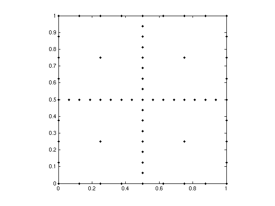
Clenshaw-Curtis sparse grid at level 4:
Exact function vs interpolant: