Polynomial Basis Functions
The piecewise multilinear approach can be significantly improved by using higher-order basis functions, specifically the Lagrange characteristic polynomials. For smooth objective functions, polynomial sparse grid interpolation achieves spectral convergence rates.
Chebyshev-Gauss-Lobatto (CGL) grid
The natural choice for polynomial sparse grid interpolation is the set of Chebyshev-Gauss-Lobatto nodes (also called Chebyshev extrema), because:
- They are well-conditioned for high-degree polynomial interpolation (Lebesgue constant grows logarithmically).
- They form a nested hierarchy: the nodes at level \(\ell\) include all nodes from levels \(0, 1, \dots, \ell-1\).
- The resulting sparse grid has the same number of points as the Clenshaw-Curtis grid.
The 1-D nodes at level \(\ell\) are
Barycentric Lagrange interpolation and the discrete cosine transform (DCT) are used internally for efficient evaluation and surplus computation.
Gauss-Patterson grid
Since version 5.0, the Gauss-Patterson sparse grid is available. It is based on the abscissae of the Gauss-Patterson nested quadrature rule, which achieves a higher degree of polynomial exactness than the CGL nodes for integration purposes. The maximum supported depth is 6.
The 1-D Gauss-Patterson nodes at level \(\ell\) include \(2^{\ell+1}-1\) nodes total (all nodes from levels \(0, \dots, \ell\) in a nested fashion).
Error estimate
Define the function class
i.e. all mixed partial derivatives up to order \(k\) in each coordinate are bounded. For \(f \in \mathcal{F}_d^k\), the CGL sparse grid interpolant \(A_{q,d}(f)\) satisfies
where \(N\) is the number of CGL support nodes. Compared to the piecewise-linear rate \(N^{-2}(\log N)^{2(d-1)}\), the polynomial basis achieves the higher rate \(N^{-k}\) for smooth functions (\(k > 2\)).
Grid point counts
The number of grid points of the CGL grid equals that of the Clenshaw-Curtis (CC) grid (see Linear Basis Functions).
The Gauss-Patterson grid has the same point counts as the NoBoundary (NB) grid.
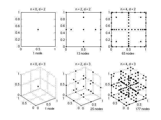
The figure below shows the CGL sparse grids at levels 0 and 2 in two and three dimensions.
When to use polynomial basis functions?
There is a trade-off between accuracy gain and the computing time required both to construct and to evaluate the interpolant. The higher-order accuracy only becomes effective with increasing number of nodes. We recommend polynomial basis functions when both of the following conditions are met:
- The objective function is known to be very smooth (analytic or at least \(C^k\) for large \(k\)).
- High relative accuracies smaller than \(10^{-2}\) are required.
For lower accuracies or functions with limited smoothness, the piecewise-linear Clenshaw-Curtis grid is generally the better choice.