Quickstart¶

Import the common constructors:

from mcerp import *

Create Distributions¶

Construct uncertain variables from probability distributions:

x1 = N(24, 1)  # normal distribution: mean 24, standard deviation 1
x2 = N(37, 4)  # normal distribution: mean 37, standard deviation 4
x3 = Exp(2)  # exponential distribution: lambda 2

The first four moments are available as properties:

x1.mean
x1.var
x1.std
x1.skew
x1.kurt
x1.stats

Calculate With Uncertainty¶

Use normal Python arithmetic:

Z = (x1 * x2**2) / (15 * (1.5 + x3))

Print the compact representation:

Z

uv(1161.35518507, 116688.945979, 0.353867228823, 3.00238273799)

Or print a labeled description:

Z.describe()

MCERP Uncertain Value:
 > Mean...................  1161.35518507
 > Variance...............  116688.945979
 > Skewness Coefficient...  0.353867228823
 > Kurtosis Coefficient...  3.00238273799

The values above may vary slightly between sessions because new samples are generated when variables are created.

Mathematical Functions¶

Use mcerp.umath for uncertainty-aware mathematical functions:

import mcerp.umath as umath
from mcerp import N

H = N(64, 0.5)
M = N(16, 0.1)
P = N(361, 2)
t = N(165, 0.5)
C = 38.4

Q = C * umath.sqrt((520 * H * P) / (M * (t + 460)))
Q.describe()

Probabilities¶

Comparison operators estimate sampled probabilities when an uncertain value is compared with a scalar:

x1 < 21
Z >= 1000

0.0014
0.6622

Discrete distributions can be queried with equality:

h = H(50, 5, 10)
h == 4
h <= 3

0.004
0.9959

For continuous distributions, exact equality usually returns zero probability:

n = N(0, 1)
n == 0
n < 0
n < 1.5

0.0
0.5
0.9332

When two uncertain values are compared, mcerp performs a paired t-test on the underlying samples to decide whether one distribution is statistically greater or less than the other.

rvs1 = N(5, 10)
rvs2 = N(5, 10) + N(0, 0.2)
rvs3 = N(8, 10) + N(0, 0.2)

rvs1 < rvs2
rvs1 < rvs3

False
True

Equality between two uncertain values checks whether they have the same root samples and therefore the same propagated moments:

Z * Z == Z**2

True

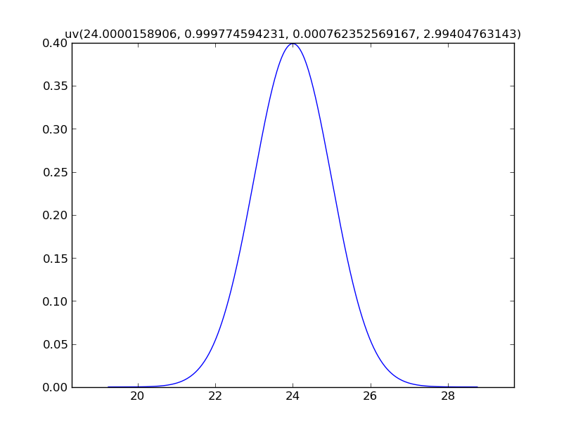
Plot Distributions¶

Plotting requires Matplotlib:

from mcerp import N

x = N(24, 1)
x.plot(show=True)

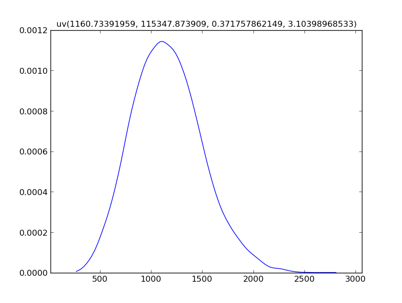
For calculated values, mcerp uses a kernel density estimate by default, because a closed-form PDF or PMF may not be available:

Z.plot()
Z.show()

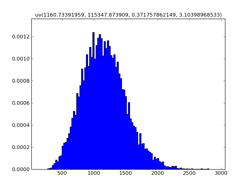
Use hist=True to show a histogram instead:

Z.plot(hist=True)
Z.show()

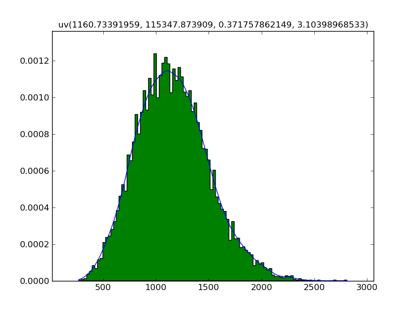
Since showing the plot is explicit, both views can be drawn together:

Z.plot()
Z.plot(hist=True)
Z.show()

Correlations¶

Use correlate before derived calculations when inputs should have a target correlation structure:

import numpy as np
from mcerp import Exp, N, correlate, correlation_matrix, plotcorr

x1 = N(24, 1)
x2 = N(37, 4)
x3 = Exp(2)

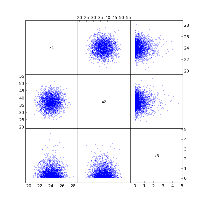
correlation_matrix([x1, x2, x3])

[[ 1.          0.00558381  0.01268168]
 [ 0.00558381  1.          0.00250815]
 [ 0.01268168  0.00250815  1.        ]]

The uncorrelated samples can be visualized with plotcorr:

plotcorr([x1, x2, x3], labels=["x1", "x2", "x3"], show=True)

Now impose a target correlation matrix:

c = np.array([[1.0, -0.75, 0.0], [-0.75, 1.0, 0.0], [0.0, 0.0, 1.0]])

correlate([x1, x2, x3], c)
correlation_matrix([x1, x2, x3])

[[  1.00000000e+00  -7.50010477e-01   1.87057576e-03]
 [ -7.50010477e-01   1.00000000e+00   8.53061774e-04]
 [  1.87057576e-03   8.53061774e-04   1.00000000e+00]]

The newly correlated samples look like this:

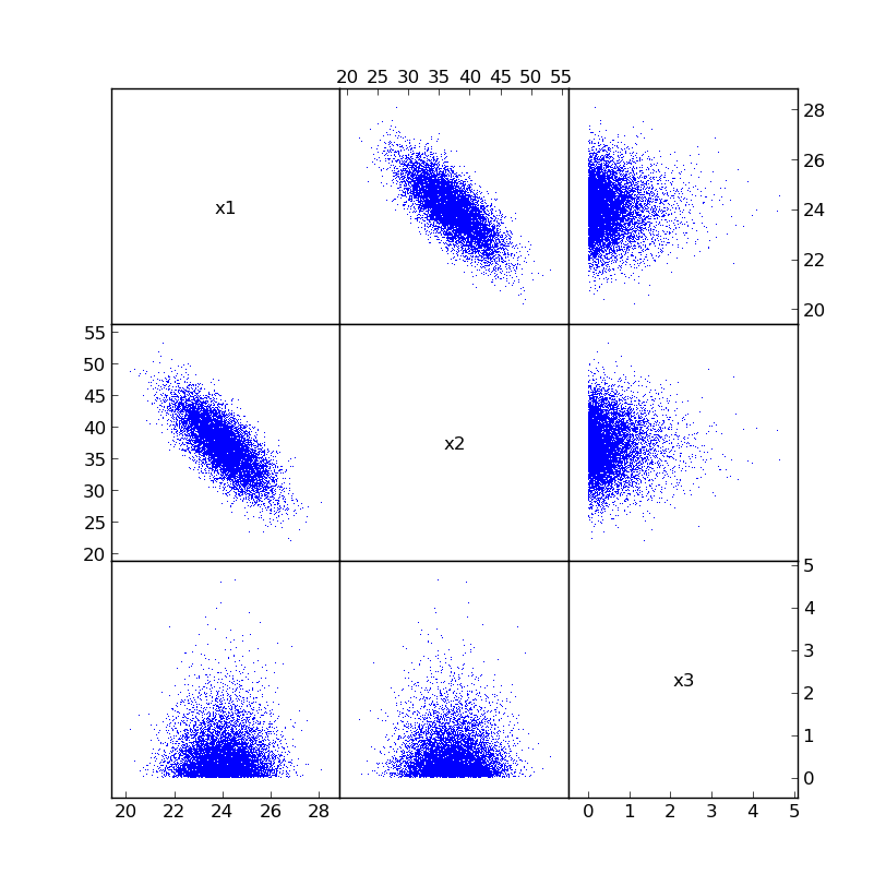
Now calculations based on x1, x2, and x3 use the reordered, correlated sample points.

Z = (x1 * x2**2) / (15 * (1.5 + x3))
Z.describe()

MCERP Uncertain Value:
 > Mean...................  1153.710442
 > Variance...............  97123.3417748
 > Skewness Coefficient...  0.211835225063
 > Kurtosis Coefficient...  2.87618465139

The correlation operation does not change the original sampled values. It reorders them so that the inputs closely match the desired correlations.

Advanced Examples¶

Volumetric Gas Flow Through an Orifice Meter¶

This engineering example propagates uncertain measurements through a gas-flow calculation:

import mcerp.umath as umath
from mcerp import N

H = N(64, 0.5)
M = N(16, 0.1)
P = N(361, 2)
t = N(165, 0.5)
C = 38.4

Q = C * umath.sqrt((520 * H * P) / (M * (t + 460)))
Q.describe()

MCERP Uncertain Value:
 > Mean...................  1330.9997362
 > Variance...............  57.5497899824
 > Skewness Coefficient...  0.0229295468388
 > Kurtosis Coefficient...  2.99662898689

Even though the calculation involves multiplication, division, and a square root, the result is close to a normal distribution: approximately N(1331, 7.6).

Manufacturing Tolerance Stackup¶

Suppose a process fits a Gamma distribution with mean 1.5 and variance 0.25. Convert those statistics to Gamma shape parameters:

k = 1.5**2 / 0.25
theta = 0.25 / 1.5

x = Gamma(k, theta)
y = Gamma(k, theta)
z = Gamma(k, theta)

w = x + y + z
w.describe()

MCERP Uncertain Value:
 > Mean...................  4.50000470462
 > Variance...............  0.76376726781
 > Skewness Coefficient...  0.368543723948
 > Kurtosis Coefficient...  3.18692837067

Because the inputs are skewed, the output remains slightly skewed.

Scheduling Facilities¶

Six station cycle times can be combined into a full process-time distribution:

from mcerp import Chi2, Exp, Gamma, N

s1 = N(10, 1)
s2 = N(20, 2**0.5)

mn1 = 1.5
vr1 = 0.25
s3 = Gamma(mn1**2 / vr1, vr1 / mn1)

mn2 = 10
vr2 = 10
s4 = Gamma(mn2**2 / vr2, vr2 / mn2)

s5 = Exp(5)
s6 = Chi2(10)

T = s1 + s2 + s3 + s4 + s5 + s6
T.describe()

MCERP Uncertain Value:
 > Mean...................  51.6999259156
 > Variance...............  33.6983675299
 > Skewness Coefficient...  0.520212339449
 > Kurtosis Coefficient...  3.52754453865

The station standard deviations help identify where consistency matters most:

for i, si in enumerate([s1, s2, s3, s4, s5, s6]):
    print("Station", i + 1, ":", si.std)

Station 1 : 0.9998880644
Station 2 : 1.41409415266
Station 3 : 0.499878358909
Station 4 : 3.16243741632
Station 5 : 0.199970343107
Station 6 : 4.47143708522

The probability of exceeding selected cycle times can be estimated directly:

[T > hr for hr in [59, 62, 68]]

[0.1091, 0.0497, 0.0083]